How To Freeze A Row In Google Sheets | Simple Guide

To freeze the rows in Google Sheets, open Google Sheets, select a row, click View from the top menu, choose Freeze, and now customize how many rows and column

Working on Google Sheets can be a very hectic process if you are working on larger datasets. To work on the larger datasets, you always have to scroll sidewise as well as down and up to complete your work.

And during working on larger datasets, it is important to keep the columns and rows visible, because if you cannot see them, you will not be able to figure out what column or row you are looking at.

To look at the rows and columns even when you are scrolling, you have to freeze the columns as well as the rows, otherwise, there are high chances of making mistakes.

But to freeze the columns and rows, you have to know how to freeze a row in Google Sheets.

If you do not know the process, you will neither be able to freeze columns, nor the rows of Google Sheets.

But if you do not know the process, do not worry. Because here in this write-up, I am going to tell you how to freeze a row in Google Sheets.

So, let’s start!

Read More: Role Of The Internet And How It Affects Our Lives

How To Freeze A Row In Google Sheets Using The Mouse

Nothing could be easier than freezing Google Sheets using your mouse. You do not have to perform even more than one step! All you need to do is take your mouse and just click the row and drag it without leaving the mouse button. That is all!

Let me explain this in detail.

Suppose, you want to freeze the top row of the dataset. To freeze this row –

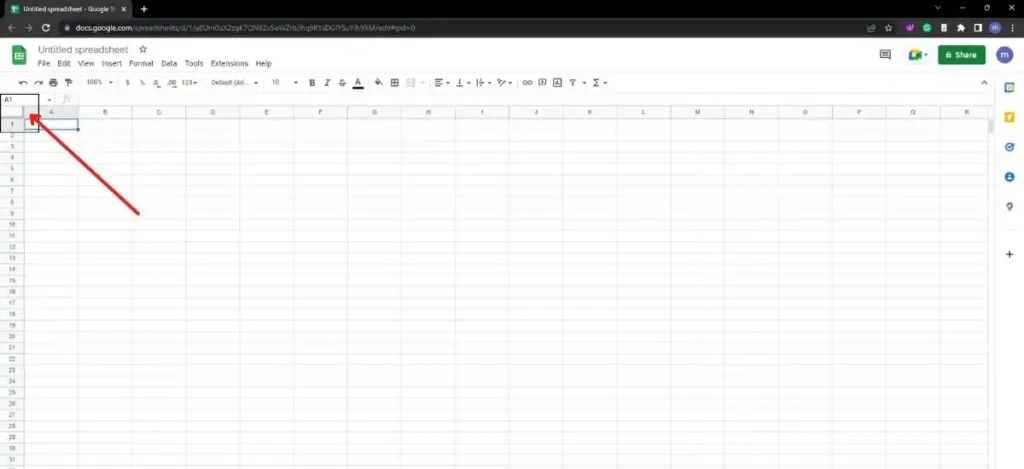
• Put the cursor on the top corner of the left side of the Google Sheet.
• Find the blank gray-colored box that has two thick lines there.
• When you take the cursor on the horizontal lines of that gray-colored box, the cursor will be changed to a hand icon.
• Now click and hold the left click button of the mouse and drag the line below the first row.
• Leave the mouse button.

You are done!

How To Freeze A Column In Google Sheets

The process of freezing the columns of Google Sheets is almost the same as the process of freezing rows in Google Sheets. The only difference is, now you have to click and drag the vertical lines instead of dragging the horizontal lines.

Let me make it clearer to you.

Suppose, you want to freeze the first column of the Google Sheet. In that case –

• Take the cursor to the left side of the top corner of the current Google Sheet.
• Find the gray-colored box with both vertical as well as horizontal thick lines.
• When you take the cursor on the vertical lines of the box, the cursor changes to a hand icon.
• Now click and hold the left button of your mouse and drag that line to the right vertical line of the first column without leaving the mouse button.
• Now leave the mouse button.

And you are done!

If you want a visual of this method, then I would like to suggest you watch the YouTube video I have given below. 

How To Freeze Multiple Rows

And now we have come to that part where I am going to tell you how you can freeze more than one row.

Actually, this is very simple too. I am giving you the steps of the process below so that you can read them and freeze any number of rows on your Google Sheet dataset.

• You have to choose any of the cells from the N-th row (N is the number of rows you want to freeze. If you want to freeze 5 rows, then you have to choose any cell from the 5^th row, if you want to freeze 9 rows, you have to choose any cell from the 9^th row)
• Now you have to click View from the menu.
• Take the cursor on the Freeze option.
• Click on the Up to current row option.

That’s it! You’re done!

How To Unfreeze Rows

There are two methods to unfreeze rows in Google Sheets. The first one is the easiest one. Just drag back the thick line from below the row to its original place which you dragged at the time of freezing the row and the row will unfreeze.

And if you want to use the second method, here it is –

• Click View.
• Take the cursor to Freeze.
• Click on No Row.

That is all!

How To Freeze Rows On Sheets For Mobile

If you are using Google Sheets on your mobile phone and you want to know how to freeze a row in Google Sheets for mobile, then read the steps below.

• Open the Google Sheets app from your mobile smartphone.
• Open the dataset you want to work on.
• Tap the spreadsheet name right at the bottom of your mobile screen. This will open the list of options for making tweaks on that spreadsheet.
• When you will tap the name of the spreadsheet, a window of options will pop up from the bottom.
• Now you will see an option for freezing rows.
• To increase or decrease the number of rows to freeze, tap the up and the down arrow buttons.
• When finished, tap anywhere out of that window. The changes will automatically be applied.

Do You Know: What is WEB 3.0?

Why Freeze Rows In Google Sheets?

When you work on larger datasets in Google Sheets, you have to continuously scroll down and right to keep working.

But while doing this, you need to keep the rows visible because if you do not get to see which row you are working at, you might end up doing a mistake.

And this is why you need to freeze the rows so that you can see them while scrolling down and right the Google Sheet.

How To Freeze Panes In Google Sheets

If you want to freeze panes in Google Sheets, just follow the steps below.

• Open Google Sheets and open the spreadsheet on which you are working. 
• Choose the row you want to freeze.
• Now click View from the top.
• From here, you can customize how many rows as well as columns you want to freeze.

You are done!

Frequently Asked Question

Q1. What is the shortcut to see all shortcuts of google sheets?

If you want to have a look at all the keyboard shortcuts in Google Sheets, then just press Ctrl + /.

A2. What is the difference between Excel and Google Sheets?

The main difference between MS Excel and Google Sheets is, MS Excel works in offline mode, and Google Sheets works in online mode. Google Sheets is meant for doing collaboration work.

Q3. What Does Freeze Row Actually Do?

If you freeze any row in a Google Spreadsheet, it becomes visible even when you scroll down or right the worksheet.

Cessation

Many people work on Google Sheets nowadays because it allows you to work in collaboration. But it is difficult to work on larger datasets as you continuously have to scroll down and right.

While doing this, it is important to keep the row and the column visible, because if you miss them, you might end up doing a mistake.

That is why people who work on Google Sheets want to know how to freeze a row in Google Sheets and that is why I wrote this article.

I hope after reading this, you will be able to freeze any row in Google Sheets on your own.

Also, Refer- How To Turn Off CC On Peacock TV?